An Electron beam writer exposes a shape by discretely scanning a focused electron beam across a primitive shape (primitives). Designers produce CAD patterns that resemble their device. These CAD patterns must be fractured or decomposed into primitives before it can be handled by an electron beam writer. Understanding the process that converts a CAD pattern into primitives provides some control over how the pattern is written.
Primitive Shapes
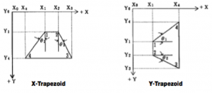
The JBX-5500FS is capable of drawing two kinds of primitive: rectangles and trapezoids. A special case of the rectangle is a square. Less obviously, a special case of a trapezoid is a triangle or a parallelogram. For the sake of clarity in the succeeding discussion, we will pretend that the JBX-5500FS has three primitives: rectangle, triangle and trapezoids. In addition, there are a few constraints on the primitives:
- At least 2 edge of the primitive must be parallel to either the X or Y axis
- The angles Θ1 and Θ2, defined in figure 1, cannot have a magnitude larger than 60°.
Other electron beam writers have their own primitives and specifications. The simplicity of the primitives allow them to be written extremely quickly.
Pattern Fracturing
CAD patterns must be fractured or decomposed into primitives before it can be handled by the electron beam writer. Most shapes can be accurately exposed by decomposing the shape into primitives. However, some shapes such as arcs, circles and narrow triangles may not be exposed as intended since they can only be approximated by primitives. Below is an example of how various shapes are fractured.
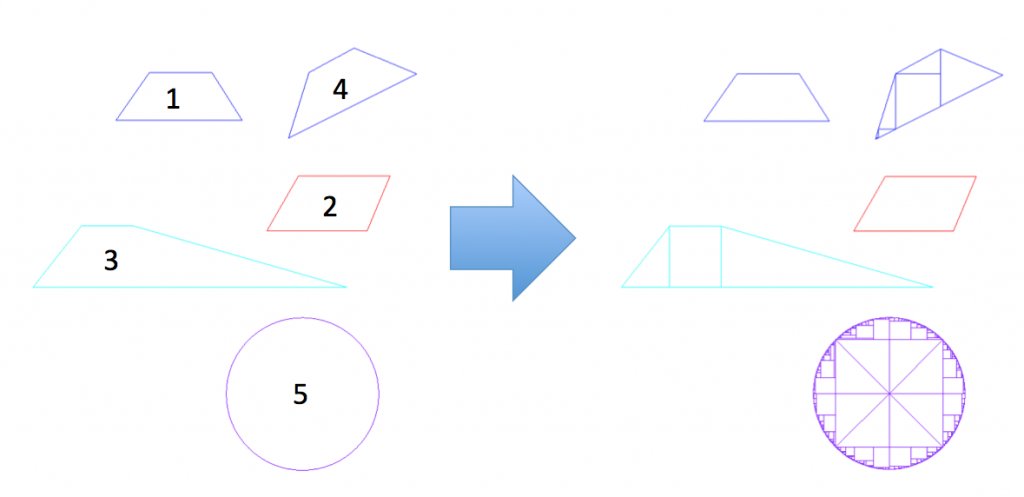
Fracturing algorithms decompose a shape by slicing horizontally and/or vertically from the vertices towards the edges. Shapes 1 and 2 are primitives so they do not need to be fractured. Primitives are typically rectangles, trapezoids and triangles for pattern generators based on a cartesian coordinate system. The slices are clearly visible in shape 3 where a trapezoid is fractured into two right triangles and a rectangle. When a shape is fractured, its constituent shapes are checked and fractured if they are not primitives. This process continues iteratively until all constituents of the original shape become primitives. Three iterations of fracturing was required for shape 4.
It is important to note that shape 1 and shape 4 are exactly the same except orientation. Since an e-beam writer scans the beam using a pair of orthogonal deflectors, namely the X-axis deflector and the Y-axis deflector, primitive shapes must share at least one edge with either of these axes. The orthogonal primitives are clearly visible in all of the fractured shapes.
A Circle, shape 5, is always approximated by CAD software that uses the cartesian coordinate system. CAD software that supports a polar coordinate system must still comply with the limitations of electron beam lithography machines using XY scanners. Thus, circles designed for e-beam lithography must always be carefully approximated as a polygon with an appropriate number of vertices along the perimeter. Fracturing circles is a tricky business and can result in erroneous exposure. The small primitives along the perimeter of the circle can cause overexposures, increasing the shape’s line edge roughness. In a severe case, the exposed pattern can look like a clover. In this case, the exposed shape will not match the designed shape due to bad layout preparation. Specialized e-beam lithography software provide a handful of fracturing algorithms that have been shown to reduce the line edge roughness of circle or shapes with round edge(s).
Fracturing Algorithms
The fracturing algorithm provided with the Jeol JBX-5500FS, shown in figure 2, is proprietary and an unfortunately unpredictable. We have developed our own fracturing algorithm designed with a simple set of rules to make it predictable. This gives the user control over the primitives from their shape.
The fracturing algorithm can be described by 3 rules:
- Trapezoidalize the shape into X trapezoids
- Trapezoidalize each X trapezoid into Y trapezoids if it is not a primitive
- Recursively trapezoidalize into X and Y trapezoids until the remaining pattern is too small
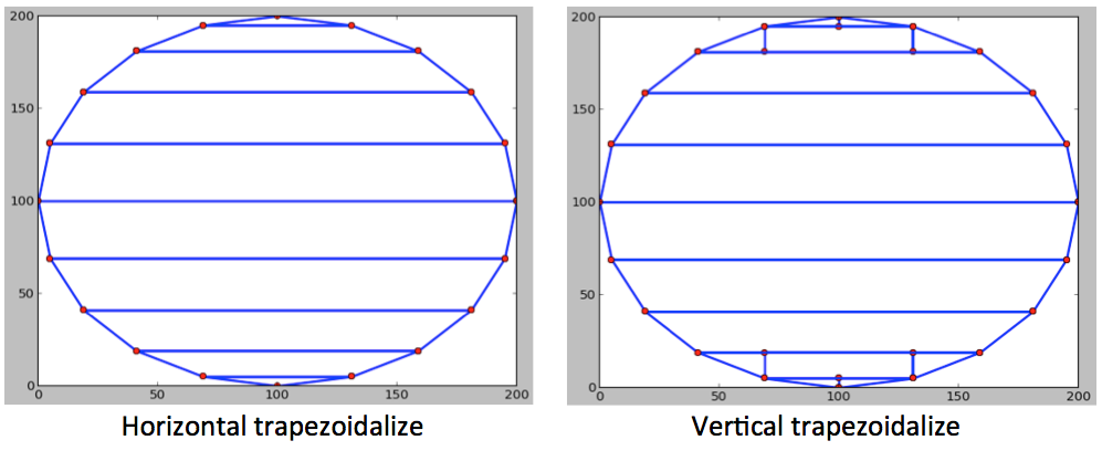
X trapezoids have bases parallel to the x axis. Y trapezoids have bases parallel to the y axis. Triangles are trapezoids where the length of one base is set to zero. Figure 3 is an example where a circle that is drawn using 20 segments is fractured. The image labeled Horizontal trapezoidalize shows the result of stage 1, where the circle is fractured along its vertices into X trapezoids. The image labeled Vertical trapezoidalize shows the result of stage 2, where the X trapezoids are further fractured into Y trapezoids. Notice that only X trapezoids with small acute angles are fractured in stage 2.
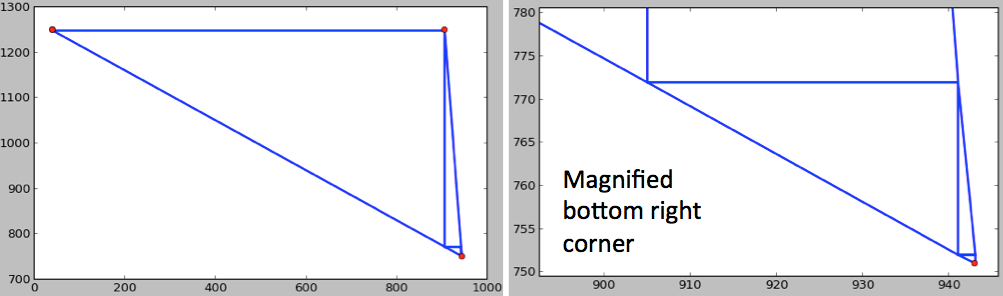
The angles within a shape is important in determining whether or not it is a primitive. Most shapes require only two rounds of fracturing to decompose it into primitives. However, shapes where neither of the adjacent edges are orthogonal to the axis may never be fully fractured into primitives. Figure 4 is an example of a shape that needs to be fractured recursively (stage 3). This shape can be fractured forever and the remaining fragment will never become primitives. Therefore, the fracturing algorithm stops when the fragments become too small to be practically exposed.
Array Fracturing
Array fracturing is a special case of fracturing which takes advantage of cell referencing and hierarchy from CAD programs. When one wants to replicate the same shape a million times on a fixed grid, it is very efficient to draw the shape only once and command the computer to repeat it. Therefore, it is extremely time and memory efficient to fracture a repeated shape only once and store it in memory only once.
The array fracturing algorithm can be described in 3 stages:
- Fracture the array if the number of rows or columns in an array is more than 2000
- Fracture the array if it crosses a field boundary along the X axis
- Fracture the array if it crosses a field boundary along the Y axis
In all stages, if fracturing must be performed, then new cells are created to store each partition of the array. At the end of stage 3, the each partitioned array will contain less than 2000 rows, less than 2000 columns and it is confined within a single write field.
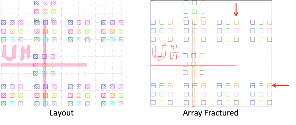
Below is a pair of images that shows the result of array fracturing. The cell contains a set of 9 squares, each square is a different datatype. The cell is referenced once at the center of the cross and once at the top of the cross. In addition, the cell is array referenced in a 2 x 4 (row x column) array. After array fracturing, some array elements that lie on a field boundary is flattened. The red arrows on the Array Fractured image indicates the position of the field boundary.
In the JBX-5500FS, array fracturing has a significant problem with writing order. For example an array element contains 10 primitive shapes and there are 1,000,000 elements in the array. The first primitive shapes will be printed for each element before the second primitive shape is printed. A significant time delay between printing each primitive will cause placement errors!